Zero order kinetics in CMBR

Environmental engineering

Problem statement

Lets consider 3 continously mixed batch reactors (CMBR) with zero-order decay kintetics (\(k_0\)) for a substance with initial concentration \(C_0\).

The parameters for each reactor are listed below:

• CMBR 1: C\(_0\) = 10 mg/L , \(k_0\) = 0.1 mg/Ls
• CMBR 2: C\(_0\) = 10 mg/L , \(k_0\) = 0.2 mg/Ls
• CMBR 3: C\(_0\) = 10 mg/L , \(k_0\) = 0.5 mg/Ls

1. Plot the concentration of each reactor as a function of time.
2. ¿What is the concentration of the substance in each reactor after 10 sec?

Solution

The concentration of a susbstance in a CMBR that decays with zero-order kinetics can be modeled as follows:

\[ C(t) = C_o -k_0t \tag{1}\]

Lets implement this equation numerically through a function:

from numpy import linspace, exp
import matplotlib.pyplot as plt

def conc(C0, k0, time):
    '''Concentration in a CMBR with first-order decay
    '''
    return C0 - k0 * time

Our function receives the initial concentration C0, the zero-order decay rate k0, and the time. We can use the same function to model the 3 CMBRs.

Note that the time variable can be either a single value of an array of values. Thus, we can compute the evolution of the concentration in a CMBR as a funtion of time.

Plot of concentration

time    = linspace(0, 20) # time in sec
k0      = [0.1, 0.2, 0.5] # zero-order decay kinetics (mg/Ls)
C0      = [ 10,  10,  10] # initial concentrations (mg/L)

for i, k in enumerate(k0):
    Ct = conc(C0[i], k, time)
    plt.plot(time, Ct, label="CMBR %i: $k_0 = %s s^{-1}$" % (i+1, k) )

plt.xlabel("time [s]")
plt.ylabel("concentration [mg/L]")
plt.legend()
plt.grid()
plt.show()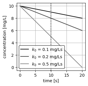

As expected from Equation 1, the concentration of each CMBR evolves linearly as a function of time, with the slope being equal to \(k_0\).

Concentration of substance after 10 sec

We can use our function considering 10 sec as the input time to ompute the concentration of the substance.

t_eval = 10 # sec

for i, k in enumerate(k0):
    conc_t = conc(C0[i], k, t_eval)
    print ("CMBR %i: C(t=%ss)= %1.1f [mg/L]" % (i+1, t_eval, conc_t) )

CMBR 1: C(t=10s)= 9.0 [mg/L]
CMBR 2: C(t=10s)= 8.0 [mg/L]
CMBR 3: C(t=10s)= 5.0 [mg/L]

Follow up questions

1. For the case of the last CMBR, what is the concentration of the substance after 20 seconds? Does the code correctly reflects the expected value?
2. Calculate the time it takes for each reactor to reach half of the initial concentration (\(t_{1/2})\)