Nth-order kinetics in a CMBR
Environmental engineering
Problem statement
Lets consider 3 continuously mixed batch reactors (CMBRs) where a substance with initial concentration \(C_0\) decays with an Nth-order rate constant \(k_n\). The parameters for each reactor are listed below:
- CMBR 1: \(C_0\) = 10 mg/L , \(n\) = 1.2, \(k_n\) = 0.1 (mg/L)\(^{-0.2}\)s\(^{-1}\)
- CMBR 2: \(C_0\) = 10 mg/L , \(n\) = 1.5, \(k_n\) = 0.1 (mg/L)\(^{-0.5}\)s\(^{-1}\)
- CMBR 3: \(C_0\) = 10 mg/L , \(n\) = 2.0, \(k_n\) = 0.1 (mg/L)\(^{-1.0}\)s\(^{-1}\)
- Plot the concentration in each reactor as a function of time.
- Compute the time required to reach half of the initial concentration in each reactor.
Solution
For a CMBR of constant volume \(V\), the concentration of a substance \(C\) that decays with a Nth-order rate constant \(k_n\) can be modeled as follows:

\[ \dfrac{dC}{dt}V = k_n C^n V \tag{1}\]
Assuming that at time \(t=0\) the concentration of substance is \(C_0\), and that \(n \neq 1\), the previous ordinary differential equation (ODE) has the following analytical solution:
\[ C(t) = \left[ C_o^{1-n} - (1-n) k_n t \right]^{\frac{1}{1-n}},\quad n \neq 1 \tag{2}\]
Note that, in this case, the concentration in the CMBR is independent of the reactor volume. Lets implement this last equation numerically through a function:
Note that our function receives the initial concentration C0, the nth-order decay rate constant kn, the order n, and the time array. We can use the same function to model the 3 CMBRs.
Plot of concentration
fig, ax = plt.subplots(figsize=(3,3)) # figure size

time    = linspace(0, 20)  # time in sec
n       = [1.2, 1.5, 2.0]  # kinetic orders
kn      = [0.1, 0.1, 0.1]  # nth-order decay rate constants (1/s)
C0      = [ 10,  10,  10]  # initial concentrations (mg/L)

for i, k in enumerate(kn):
    Ct = conc(C0[i], k, n[i], time)
    col = str(i*0.25)
    ax.plot(time, Ct, color=col,
            label="$k_n$ = %s (mg/L)$^{%1.1f}$s$^{-1}$" % (k, 1-n[i]))

ax.axhline(5, color='k', ls=':')
ax.set_xlabel("time [s]")
ax.set_ylabel("concentration [mg/L]")
ax.legend(edgecolor='k', fontsize=9)
ax.grid()
plt.show()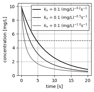
As expected from Equation 2, the concentration of each CMBR decays with the given order as a function of time. We additionally plot an horizontal line at half the concentration for each reactor (\(C = 5\) mg/L), to visually inspect the required time to reach this concentration.
Computation of \(t_{1/2}\)
We can use Equation 2 to derive the required to reach half ot the concentration in the CMRB: \[ \frac{C_0}{2} = \left[ C_o^{1-n} - (1-n) k_n t_{1/2} \right]^{\frac{1}{1-n}} \]
\[ t_{1/2} = \dfrac{C_0^{1-n}(1-\dfrac{1}{2^{1-n}})}{(1-n)k_n} \tag{3}\]
We implement the following function to compute this value:
We use the function halftime() to compute the half-times for each CMBR:
Follow up questions
- From Equation 1, verify that the dimension of the zero-order constant is [\(M^{1-n}L^{3(n-1)}T^{-1}\)].
- Show at the zero-order kinetic equation is a special case of the nth-order when \(n=0\).
- Verifiy that \(t_{1/2} = 1/(C_0k_2)\) for a 2nd-order decay reaction in a CMBR (\(n=2\)).
- Compute the concentration in each CMBR after 20 s.